.ALF, .LIN and .LIM files: ALF, LIN and LIM files are used to feed back the parameters from intmer.xls into Open Genie.  Example files can be downloaded here.  The ALF file is used to ensure that the DCS file oscillates around the SLF file.  Therefore when SLF is subtracted to give i(Q), this oscillates around 0.  The .LIN file allows you to carry out a linear correction if the .DCS data is at a slope to the .SLF data. The LIM file is used to set the limits over which each bank is used in merging the data together.

 For the .LIM file, it is best to pick a point, either at the top or bottom of an oscillation (if the data is from a glass) or in between Bragg peaks (for a crystal), as at these points the change in intensity is slower, this is preferable, because if the two banks being merged do not match up, large discontinuities will appear in the data.

INTERFERE

Once the ALF and LIN files have been written, they are used to subtract the self scattering to leave the distinct scattering.  The outputted GEM19000.INT file contains the distinct scattering i(Q) from the sample for each bank, and this can now be used to get a final, merged spectrum.

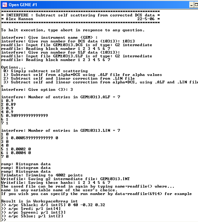
Interfere

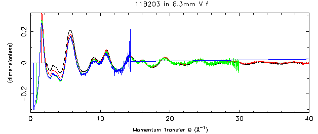
Interfere-plot

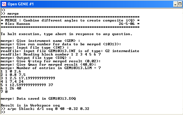
 MERGE

Once Interfere has been run, the output banks will oscillate around 0.  Once this is achieved, MERGE is used to generate a single file with a maximum possible Q range. 

If you have difficulty generating a nice .SOQ file, it is suggested only two flags in the .lim file is turned on at a time (6 and 5).  Then run merge and plot the result and looking to see if the data have been merged nicely, or if there a sharp discontinuities present.  If sharp peaks do occur, the limits will need to be changed.  When satisfied, add in another section and rerun merge.  Repeat until all the banks you wish to use are added in.  The final file will be a .SOQ file. 

Merge

Merge-plot

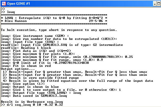
LOWQ 

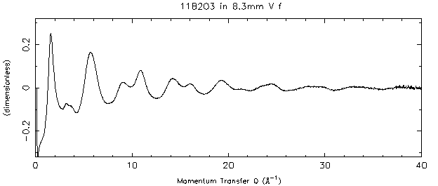
After merge, distinct scattering data from ~0.5 Å out to 40-50 will have been made.  All that remains is to fill in the low Q data, down to 0 Å. This is achieved by fitting a quadratic to the low Q portion (between ~0.5 – 1).  I normally use the quadratic instead of the data, starting at the upper limit, however the program offers you several options.  The output can be saved as a binary file and is automatically stored in an Open Genie workspace, soq_lowq.

LowQ

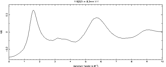
LowQ-plot

The LowQ plot is the final i(Q) data.  For information on Fourier transforming the data to produce a correlation function, such as T(r). See the 'Producing and analysing correlation functions' web page​