Install Mantid Workbench

Download from: https://download.mantidproject.org/

O. Arnold, et al., Mantid—Data analysis and visualization package for neutron scattering and μSR experiments, Nuclear Instruments and Methods in Physics Research Section A, 764 (2014) 156-166, http://dx.doi.org/10.1016/j.nima.2014.07.029

Part I
- Organize a Batch File
- Setup Mantid
- Reduce Data

Part II

- Manage plots

Part III
- Add runs
- Use event mode
- Slice wavelength ranges

Part IV
- Merge small and high angle
- Use Algorithms
- Run a Python Script

Part II:

After reducing your data using the ISIS SANS Reduction Graphical User Interface (GUI) in Mantid Workbench...

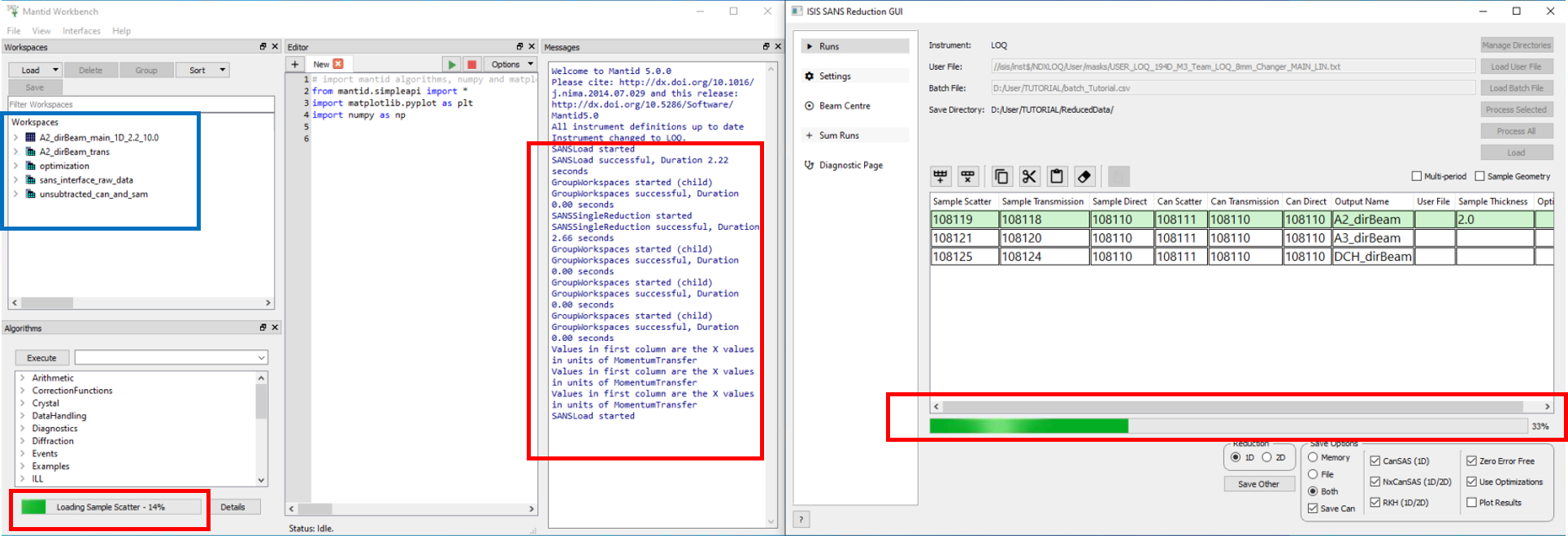
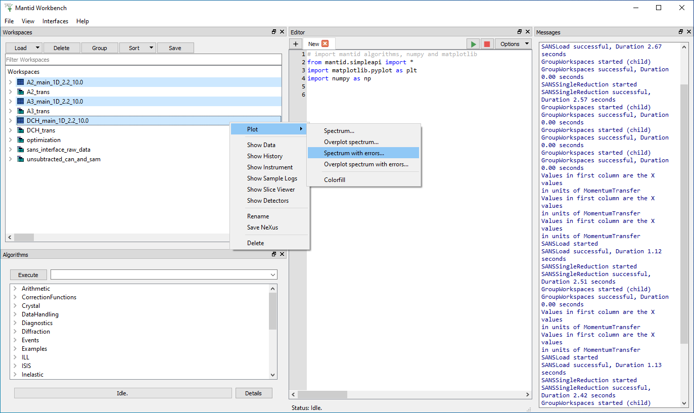
The green bar on the bottom indicates the progress of the process. You can now minimize the SANS Reduction GUI window and continue to monitor the process through the main window of MANTID WORKBENTCH. In this window you can also monitor the Messages during the reduction process, manage plots in Workspaces, use pre-existing Algorithms and run Python scripts using the Editor.

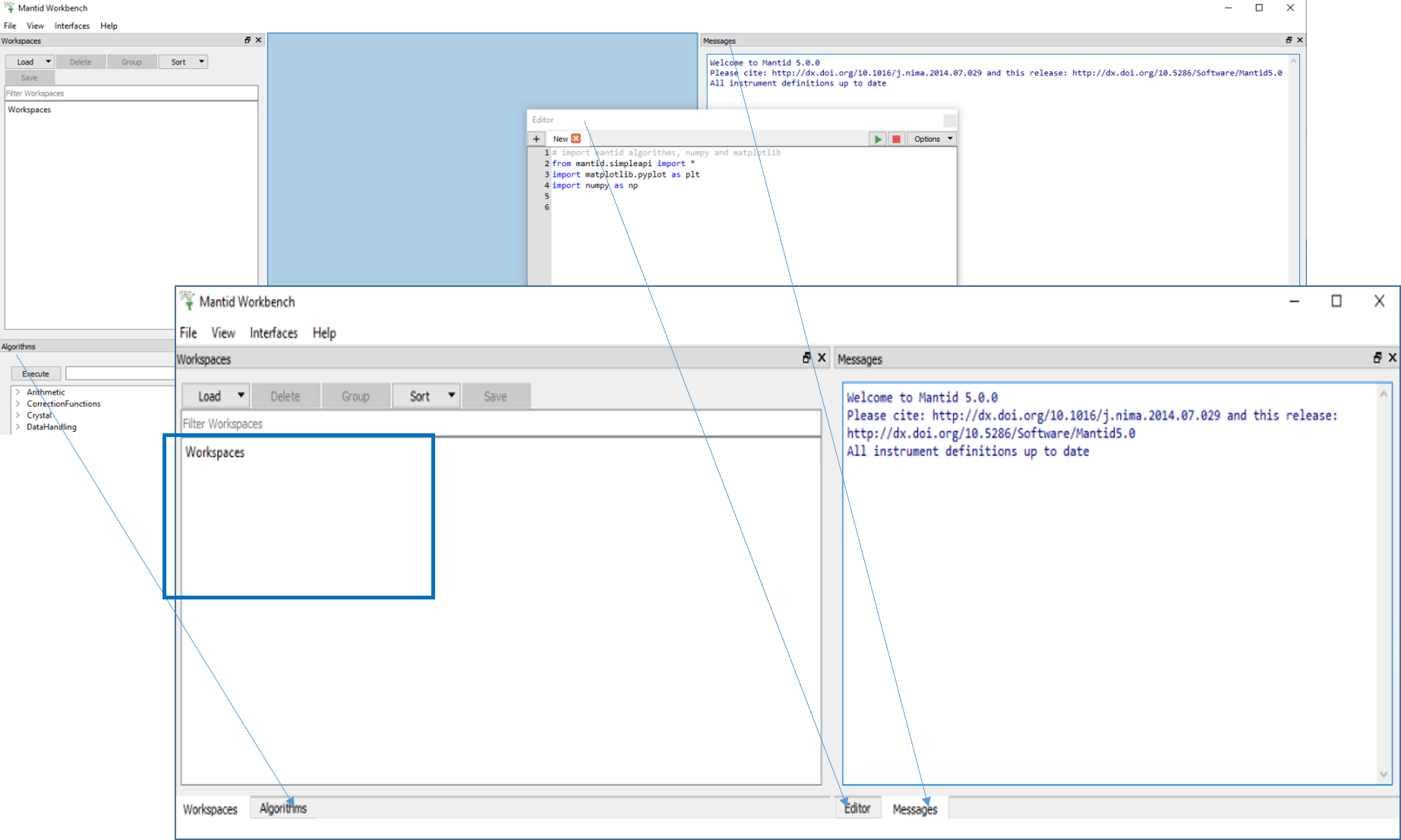
You can organize/hide these areas (Workspaces, Algorithms, Editor and Messages) as you want. Here, in the picture below, there is one examples how to drag one behing the other and organize them as tabs:

The reduced data is collected in the WORKSPACE WINDOW highlighted in blue in the pictures above.

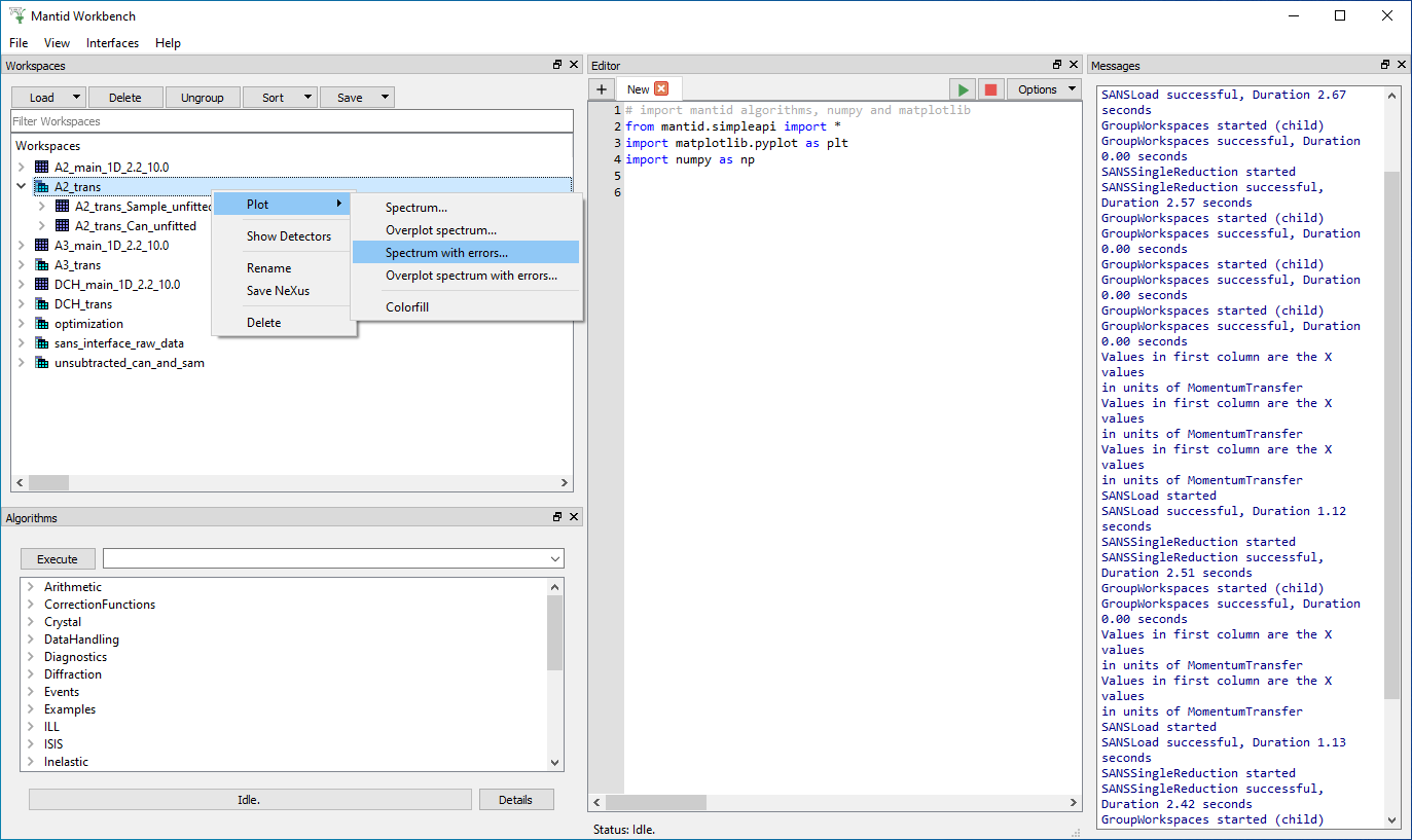
Check if the transmission data are ok by clicking on “A2_trans” in Workspaces, then right click on your mouse “Plot > Spectrum with errors” as in the picture above.

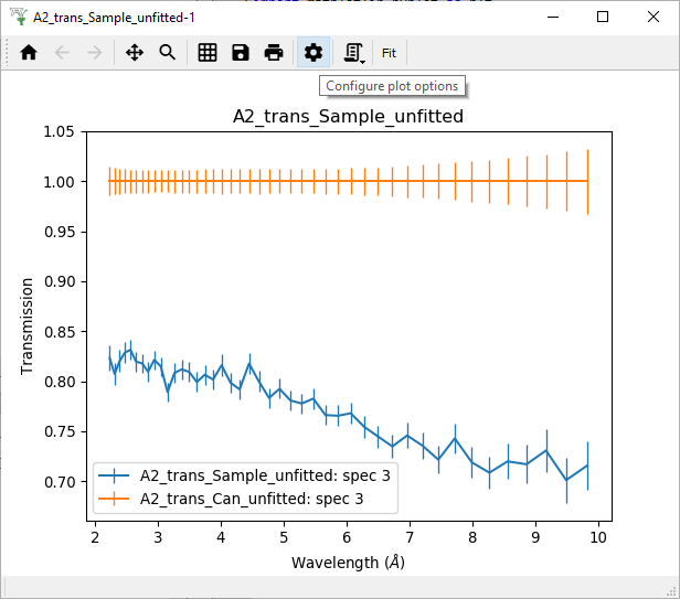
This graph shows that the transmission of the Empty Beam (we have used the Empty Beam, i.e. no sample, as the “Can” for this Sample reduction) is always 1 (or 100%) as it should be. And the transmission of the sample A2 varies with the wavelength from 85% to 70% in this example above.

To modify axes, labels, colour of the lines, etc, click on the COG WHEEL to “Configure plot options":

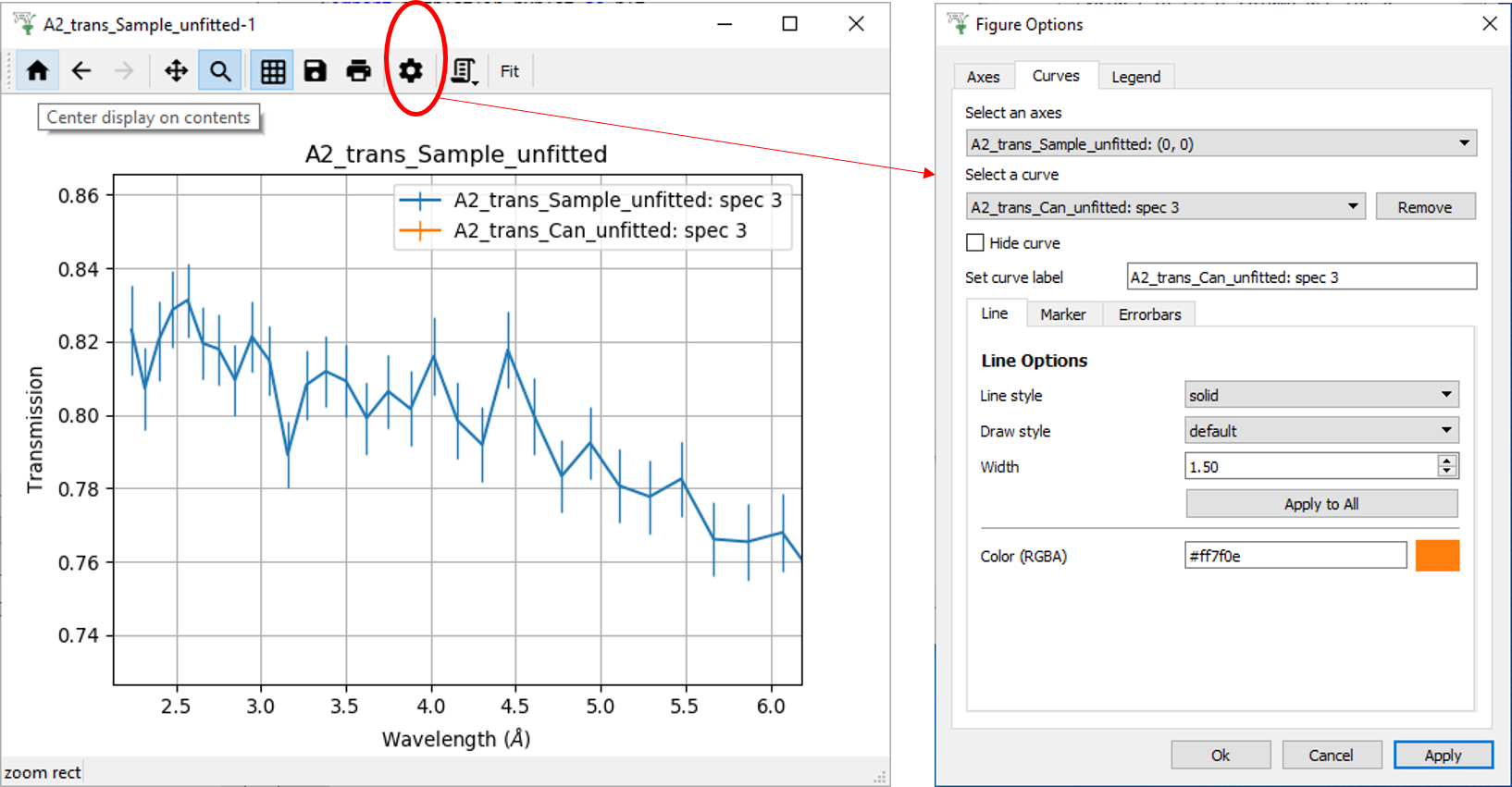
For ZOOMing on part of the graph, click on the magnifying glass icon; to unZOOM, click on HOME icon. There is also a GRID icon beside the magnifying glass icon to toggle grid/normal view.

Use CONTROL+click to select more than one curve to plot as in the figure above. Right click with your mouse to Plot > Spectrum with errors as in the picture above.

Right click with your mouse to choose Axes > Log x / Log y.

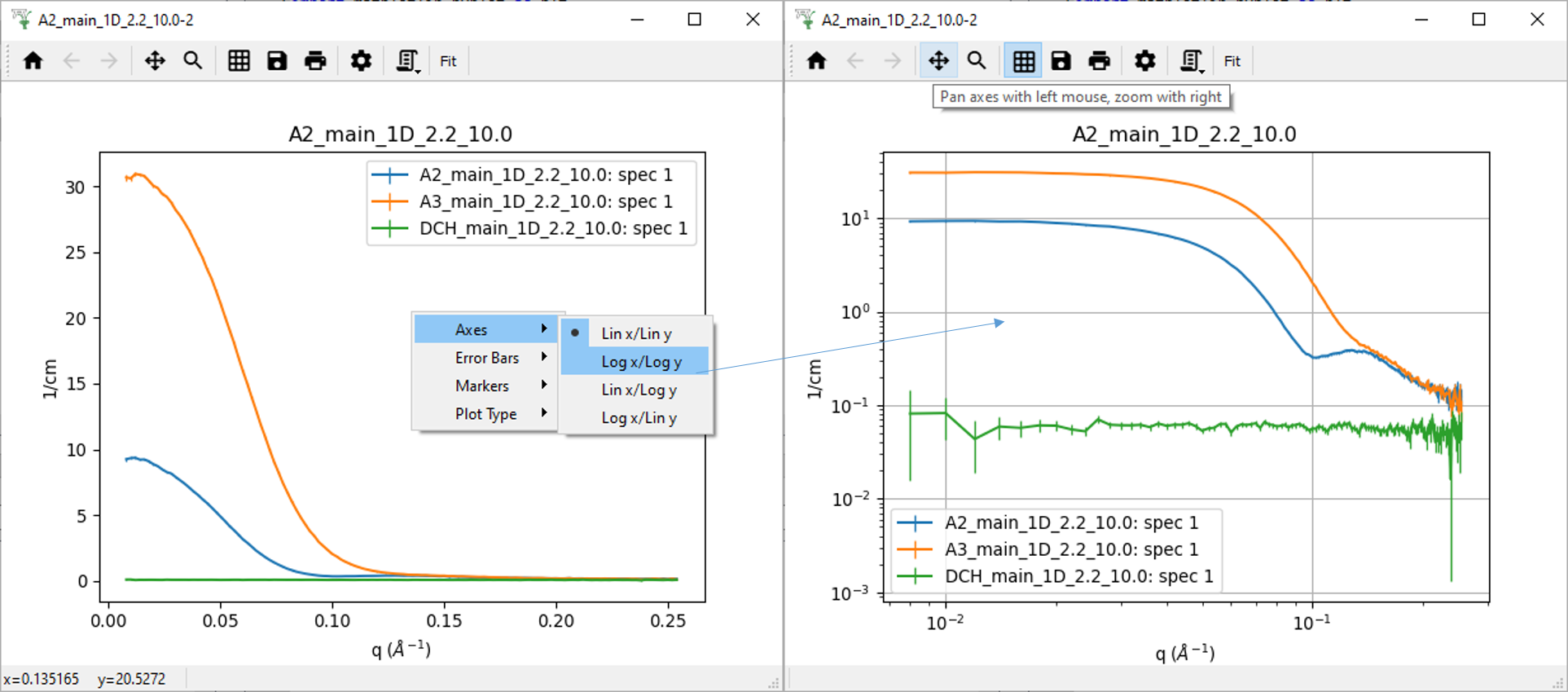
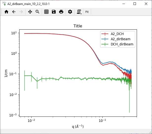
Here we plotted all curves without subtracting the background. The subtraction can be done using the Mantid algorithms (learn more in Part IV) or directly from the SANS Reduction GUI as in the example below:

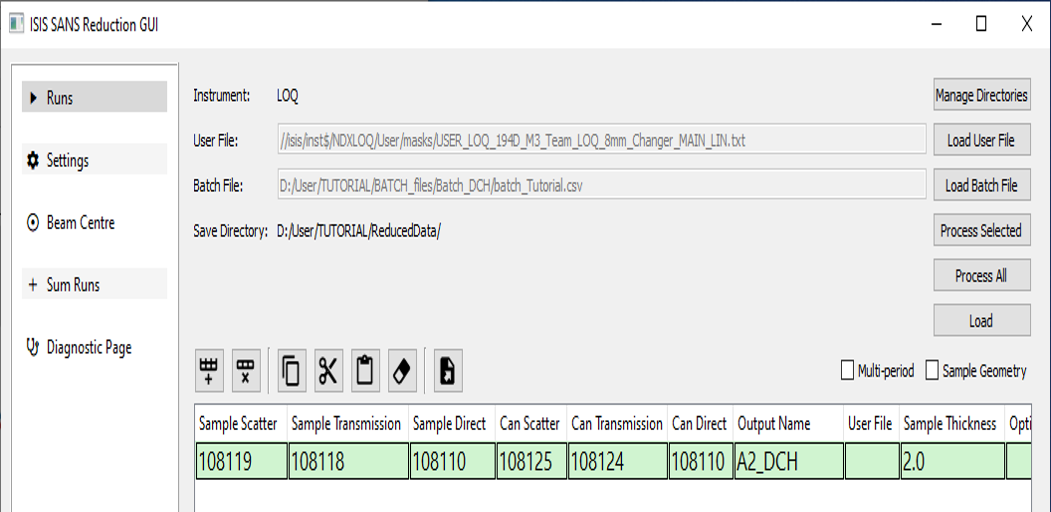
As explained in Part I, fill in the SANS Reduction GUI or the Batch File, but this time changing the Can run numbers to subtract a background sample (water, buffer, sample cell…). Here, we use the DCH sample as the “can", and so we are subtracting DCH from A2, then the reduced file will be called “A2_DCH".